Query an Analytic View in an Excel worksheet
The Query Wizard menu enables you to query an Analytic View and retrieve the results in an Excel Worksheet. Once the wizard retrieves the data, it becomes local to Excel. You can further edit the data in Excel but not write back to the Autonomous AI Database.
This menu is unavailable if you install Oracle Autonomous Database for Excel using the Microsoft Store.
You can query an Analytic View to visualize the result data in the worksheet. You can search for the Analytic View, and select measures, hierarchies, and levels from the query. You can also add filters and calculated measures to the query and view the query result in the spreadsheet.
By default, the data is retrieved in tabular format. You also have the option to create an Excel pivot from this data.
The Query Wizard has three panels:
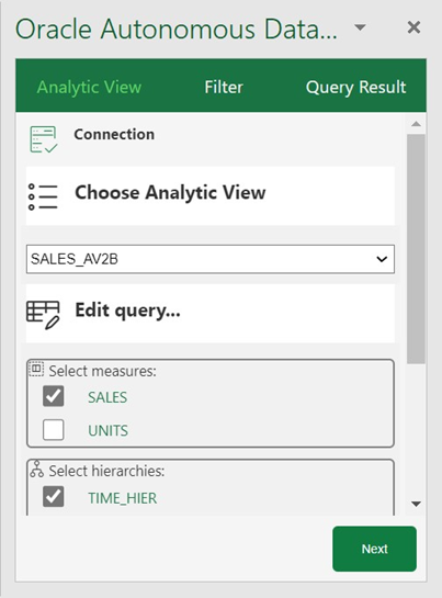
- Analytic View panel:The Analytic View panel contains a list of Analytic Views from which you build queries. You edit the query by selecting
- measures
- hierarchies,
- and levels
and progress to the next panel.

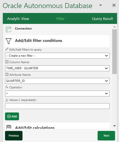
Description of the illustration av-new.png - Filter panel: The Filter panel displays to the right of the Analytic View panel when you click Next on the wizard. You can create filter conditions to filter the data and also add manual calculations to the Analytic View query in this panel.

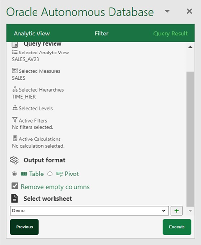
Description of the illustration filter-new.png - Query Result panel:When you click Next on the wizard, the Query Result panel displays to the right of the Filter panel. You run the query once you select the filter criteria and determine what calculated measures to add to your query. You can view and revise the SQL query. After the SQL query runs, you view the query results in the worksheet. You can select the output format of the result here. You can view the results in tabular format or a Pivot table.

Description of the illustration query-result-new.png
To query an analytic view and explore the Query Wizard menu in the MS Excel ribbon:
- On the ribbon, select the Query Wizard icon.
- Selecting the Query Wizard opens an Oracle Autonomous Database dialog box in the Excel Task Pane.
- Select an existing Analytic View from the drop-down in the Analytic View pane. As you select the Analytic View, it appears on the Analytic View field.
- Select your choice of measures, hierarchies, and levels the available measures, hierarchies and levels associated with the Analytic View. Click Next.
- The wizard window progresses to the Filter pane where you can add or edit filters to query.
- Under Add or Edit filter conditions, do the following.
- Select the column name and the attribute name from the drop-down- the values of the attribute change dynamically with the change in column names.
- Select an operator in the Operator field to apply to the values that you specify in the Value field.
- Specify a value or values from the list containing your selected column members. You need to enter the value into the Values field manually. For example, you can select > in the Operator field to use only values greater than the value that you select in the Value list. If you select 100,000 from the Value list, the filter uses values from the column greater than 100,000. You can use this information in an analysis to focus on products performing well. For multiple values use “:” as the separator.
- Click Add Filter to add another filter condition.
- Under Add or Edit Calculations, do the following.
- Specify the column whose values you want to include in the group or calculated item.
- On the Calc expression field, enter a custom calculated expression you want to perform on the column value. You can add functions or conditional expressions.
- Click Next to progress to the Query Result.
- You can view, edit, and review the query you have generated from the Query Review editor.
- Select Remove empty columns to remove columns with no values returned in the result.
- Select Column per level to retrieve all hierarchy levels in a single column.
- Select the worksheet from the drop-down where you want to view the result.
- Click Execute to run the query.
- You can view the result of the query in the worksheet you select.
- You can always modify the query in the Oracle Autonomous Database dialog box editor even after results are generated.
- Select Table in the Query Result pane to view the results in the worksheet in a tabular format.
- Select Pivot in the Query Result pane to view the results in a new worksheet in Pivot format.
View the results in Pivot tables
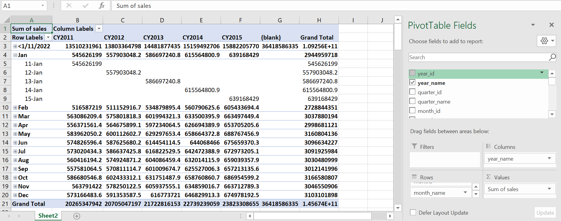
A Pivot table view is interactive and allows you to transpose rows and columns. A pivot table can summarize, sort, reorganize, count the total and perform an average of the result data. They are navigable and drillable.
Apart from tabular mode, to view the query results in pivot table mode, select the Pivot Table option in the Autonomous Database wizard. Click Run to view the query results in the Pivot table.
Clicking Run opens the query results in a new sheet with a PivotTable Fields wizard.
Parent topic: Oracle Autonomous Database for Excel
